

Last week, the DNA of 6 parents (154, 156, 1136, 1187, 2066, and 2156) was extracted. This week, these samples were diluted in order for later use in polymerase chain reaction (PCR). Each PCR plate (10 plates in total) contained all 6 parents. To better understand, 3 microliters of parent 1 (154) were placed in the first row across (A 1-12). Parent 2 (156) was placed in the second row across (B 1-12). This pattern continued until parent 6 (2156) was placed in F 1-12. Consequently, sample designation was coordinated with the PCR plate being placed horizontally instead of vertically. After all diluted DNA was distributed in this pattern across all 10 plates, the cocktail solution was made.
For the cocktail solution, distilled water, 10x buffer, DNTPs, Taq polymerase, forward primers, and reverse primers were combined. It is important to note that different forward primers (FR) and reverse primers (RM) were used for each PCR plate. Consequently, the cocktail solution had to be repeated for each plate with distinct primers. To better understand, plate 1 utilized FR 7475 and RM 2067 while plate 2 utilized FR 7677 and RM 2067. Once plate 7 was reached, RM changed to 2068 and FR to 8687. RM 2068 remained until plate 10. Additionally, the calculation of the amount of cocktail solution for each plate was centered around knowing that there will need to be enough for 74 wells. Extra is also needed so this led to Ate Eva calculating for 75 samples. Into each PCR well went the 6.8 microliters of designated cocktail solution and 8 microliters of mineral oil.


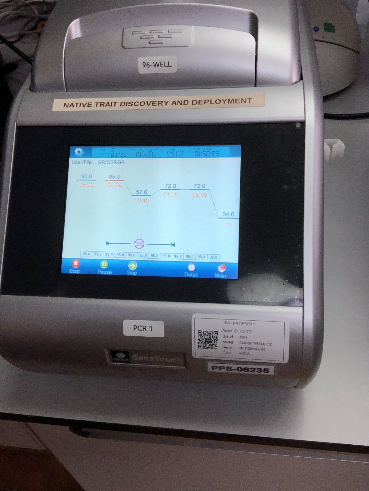
These plates were then put into separate PCR machines. After inserting a plate into the PCR machine, one needs to choose the following options: run, 57 °C, SSRGR, sample volume = 10, block, and save.
While these plates ran for around an hour and 20 minutes, the gel solution for electrophoresis was prepared. For the gel solution, 1x TBE, syber DNA gel stain, and condalab agarose gel were combined into a 1000 ml pyrex erlenmeyer flask. The flask was then heated in the microwave for 6 minutes. After this heating, the solution was observed to be bubbling. While it cooled down, combs were placed into casting racks. The solution was then poured from the middle of the casting racks and then it began to disperse itself. One needs to make certain it is evenly distributed and then covered with aluminum foil. Once the gel completely solidified, all combs were removed and wells became visible.

To prepare for the loading of the gel, 2 microliters of loading dye was added to each PCR well. Also, 3 microliters of ladder was pipetted into the first and last well of the gel. After each row (parent), the pipette tip was washed to ensure no contamination occurred. The gel then ran for 45 minutes at 170 volts.


For the screening of the gels, a Quantum VILBER machine was used. Each gel was laid long ways or horizontally and then the following options on the computer screen were chosen: auto, 90 degrees, and crop. The brightness of the image was also increased and then each image was saved to the desktop with a label (ex. plate1 RM 2067, 7475FR 6/21/23 57 temp). Then, the gel would be removed and the machine wiped down with a kim tech wipe.

Zinc and yield are negatively correlated traits. The crossing of 2 parents (trait of high yield) with 4 donor parents (trait of high zinc), aims for these 2 traits to be positively correlated. From the gels, we aim to see parental polymorphism or rather signal of samples being heterozygous. Thus, 2 bands should be present. However, when looking at the gels only plate 2 seems to contain heterozygous samples. All other plates demonstrate single bands. Consequently, more backcrossing needs to occur to create a better fixed generation.

During this third week at IRRI, I visited head house with Ate Eva. This is where the threshing, dehulling, and seed sorting of some rice samples occurs. I was able to complete these processes with brown rice and long-grain white rice samples. Threshing is when the grain is separated from the panicle. This is often done manually with the use of a wooden knife or it can be completed by a machine. After this step, comes dehulling. It is when the husk is removed from the seed. I did not witness anyone completing this step manually. If a machine was utilized for a sample, it is cleaned before the next sample goes in. This is to prevent any contamination between strains. On one of the walls of the head house are many photos of the biofortification team. I enjoyed seeing each one because this gave me a glimpse into the type of work environment that has been cultivated here at IRRI. One of friendship and teamwork.


In order to analyze data for the identification of lines with high yield and high zinc, Ate Nirusha conducted linkage disequilibrium (LD) pruning. Linkage disequilibrium measures non-random single nucleotide polymorphisms (SNPs). These non-random variants are concluded to have high LD, are often close to one another, and reveal similar information. On the other hand, random SNPs characterize regions that are recombinant. These random variations are concluded to have low LD, are often far apart, and reveal different information. Ate Nirusha wants to find a region of interest in the genome (quantitative trait loci) that has a direct influence on high zinc and yield. Finding such a region is easier with LD pruning because this process allows for the removal of non-random SNPs. Thus, random SNPs/ markers are left which do not pass a certain threshold called R-squared (calculated from allele frequency, 0.5 thresholds utilized by Ate Nirusha). The creation of an LD decay plot is also helpful because it demonstrates the genetic distance between markers. As genomic distance increases between markers, LD decreases. Therefore, random SNPs are better able to be pointed out. An L-shaped curve is very common for an LD decay plot. Although Ate Nirusha is pruning the data, the number of markers should still remain around 55,000. After pruning, RapDB was utilized to look for genes. This program allows one to search by chromosome, enter coordinates for a specific locus, and include keywords. Ate Nirusha believes that there may be a quantitative trait loci (QTL) on chromosome 6. So, chromosome 6 was chosen, coordinates were entered, and keywords such as meta-homeostasis, meta-transport, zinc-iron binding, zinc, and iron were typed in. However, the results were extensive and consequently signified that more LD pruning needed to occur.
I also had the opportunity to continue working with Ate Hsu and learning about their heat stress experiment. Some obstacles had been encountered by the glass house samples. The glass house had been frequently becoming too hot, indicating a possibility that the plants could be subjected to heat stress too early. Heat stress is not to be experienced by the plants until August 15 when the plants will reach the budding stage. Consequently, fans were now routinely turned on during the day. Also, many of the plants began to demonstrate a yellow discoloration of the leaves. Some samples were sent to the pathogenic division of IRRI and the results indicated that maggots had been infesting the plants. Bulldock insecticide was applied to the plants.

Due to the various lines having different flowering dates, strains with late flowering dates were consequently transplanted first in order for the coordination of all strains to have the same heading date. This is so that heat treatment can be applied at the same time. On 6/22/23, parents and progenies with flowering dates of or near 83 days were transplanted. From each line, the 8 strongest (tall/wide panicles) were chosen. 4 pots, filled with soil and fertilizer, were designated for each line. 2 plants per pot, and the strongest was placed in the middle and the other near the edge. One can identify the parents by looking at the labeling stick placed in each container/pot. The full name of the parent strain will be written (ex. SwarnaSub1, IR2006-P12-12-2, IRRI 154, Dasan, IRRI 156, Milyang-23, Giza 178). On the other hand, the progenies which resulted from the crosses are labeled with NS, followed by a designation number for that specific line, and then followed by a number that is specific to the plant itself (ex. NS 1751-1, NS 1751-2, NS 1751-3, NS 1751-4). Looking at this experiment from a wider perspective, it is vital to note that Ate Hsu needs 2 seasons in the field for confirmation of accurate data. As of now, Ate Hsu has completed 1 season in the field and is in the process of completing 1 controlled season. The second field season will be harvested around November. This gives me insight into how long the process of data collection is and how such organized efforts are important for accurate conclusions.


The IRRI Gene Bank monitors seed viability every 5 years (for short-term storage). If the viability of seeds falls below 85, then there is a need for field work and agro-morphological characterization. I was able to visit the viability testing of rice strains Sativa (from Asia) and Glabirmia (from Africa). Seeds are raised in seed beds and then after 21 days, they are pulled. The following day, they are transplanted. In terms of the organization of strains in the field, each strain is placed in 5 rows. Also, each plant has to be cut from the top in order for the strand to grow straight after transplanting. Irrigation pipe systems provide water to the plants. Characterization begins at the late vegetative stage. At the post-harvest stage, some examples of characterization include amylose, gel consistency, and gelatinization. Also, harvest days are highly variable due to some strains being more or less photosensitive than others (100-160 day range).


I appreciated learning about the confirmation process of parental polymorphism, LD pruning, coordination of flowering dates in an experiment, and field seed viability testing.